Starbucks Capstone Project Blog
- Project Overview
- Data Preparation
- Data Exploration
- P_testing Offer Effectiveness
- Offer Classification
- Offer Decision Making
- Conclusion
Project Overview
As part of my Udacity Capstone project, I have to write a blog post detailing my work on the problem. This is that post.
The aim of the project is to develop a strategy for giving offers (like discounts or bogoffs) to user of the Starbucks rewards app.
The main way this will be done is building a classification model to determine the likelihood of a user viewing or completing an offer. Ideally we would also try to estimate how a user’s spend would be impacted by an offer, or combination of offers, unfortunately this does not appear to be a tractable machine learning problem. At least with the data available.
Treating this as a classification problem is a very natural approach. It also offers a lot of flexibility and be easily combined with subsequent work on other aspects of the problem.
The data set is imbalanced, particularly the viewed/not viewed classes, and so performance of the model will be measured by it’s f1-scores on each class. Since the model will be used to output estimates of probabilities it is important that the model performs well on both positive and negative classes.
The strategy itself will need real world testing to evaluate. There is some discussion of this in the conclusion.
The code and datasets for this blog are available here.
Data Preparation
Offers
The offers that Starbucks sent out are as follows. The reward is the value of product for a bogoff and value of the discount otherwise. Similarly the difficulty is the required spend to complete the offer.
The data is contained in the file portfolio.json which has the following schema.
- id (String) - offer id
- offer_type (String) - type of offer ie BOGO, discount, informational
- difficulty (Int) - minimum required spend to complete an offer
- reward (Int) - reward given for completing an offer
- duration (Int) - time for offer to be open, in days
- channels (List of Strings)
Dummy variables were used for the channels and the offers were given a simplified name, resulting in the following portfolio.
| Offer ID | Reward | Difficulty | Duration | Offer Type | Mobile | Social | Web | Name | |
|---|---|---|---|---|---|---|---|---|---|
| 9b98b8c7a33c4b65b9aebfe6a799e6d9 | 5 | 5 | 7 | bogo | 1.0 | 1.0 | 0.0 | 1.0 | bogo,5,5,7 |
| f19421c1d4aa40978ebb69ca19b0e20d | 5 | 5 | 5 | bogo | 1.0 | 1.0 | 1.0 | 1.0 | bogo,5,5,5 |
| ae264e3637204a6fb9bb56bc8210ddfd | 10 | 10 | 7 | bogo | 1.0 | 1.0 | 1.0 | 0.0 | bogo,10,10,7 |
| 4d5c57ea9a6940dd891ad53e9dbe8da0 | 10 | 10 | 5 | bogo | 1.0 | 1.0 | 1.0 | 1.0 | bogo,10,10,5 |
| fafdcd668e3743c1bb461111dcafc2a4 | 2 | 10 | 10 | discount | 1.0 | 1.0 | 1.0 | 1.0 | discount,2,10,10 |
| 2906b810c7d4411798c6938adc9daaa5 | 2 | 10 | 7 | discount | 1.0 | 1.0 | 0.0 | 1.0 | discount,2,10,7 |
| 2298d6c36e964ae4a3e7e9706d1fb8c2 | 3 | 7 | 7 | discount | 1.0 | 1.0 | 1.0 | 1.0 | discount,3,7,7 |
| 0b1e1539f2cc45b7b9fa7c272da2e1d7 | 5 | 20 | 10 | discount | 1.0 | 0.0 | 0.0 | 1.0 | discount,5,20,10 |
| 3f207df678b143eea3cee63160fa8bed | 0 | 0 | 4 | informational | 1.0 | 1.0 | 0.0 | 1.0 | informational,0,0,4 |
| 5a8bc65990b245e5a138643cd4eb9837 | 0 | 0 | 3 | informational | 1.0 | 1.0 | 1.0 | 0.0 | informational,0,0,3 |
Events and Offers
All the events - offers received, viewed or completed as well as transactions are recorded in a single file - transcript.json. The columns available were
- event (String) - record description (ie transaction, offer received, offer viewed, etc.)
- person (String) - customer id
- time (Int) - time in hours since start of test. The data begins at time t=0
- value - (Dict of Strings) - either an offer id or transaction amount depending on the record
The rows of the frame look like the following:
| Person | Event | Value | Time |
|---|---|---|---|
| 78afa995795e4d85b5d9ceeca43f5fef | Offer Received | {‘offer id’: ‘9b98b8c7a33c4b65b9aebfe6a799e6d9’} | 0 |
| 389bc3fa690240e798340f5a15918d5c | Offer Viewed | {‘offer id’: ‘f19421c1d4aa40978ebb69ca19b0e20d’} | 0 |
| 9fa9ae8f57894cc9a3b8a9bbe0fc1b2 | Offer Completed | {‘offer_id’: ‘2906b810c7d4411798c6938adc9daaa5’} | 0 |
| 02c083884c7d45b39cc68e1314fec56c | Transaction | {‘amount’: 0.8300000000000001} | 0 |
Most of the pre-processing for the model was needed here.
These needed to be assembled into frames for each event and were then aggregated further. Transactional information like mean spend, total spend and number of transactions was gathered and merged with the user data. It was also often necessary to pull this data for specific time periods. For example getting total spend during the period that a given offer was active.
Some care was needed to match up offers received by a user to subsequent events like viewings or completions. A user might receive the same offer twice across the month, so it was necessary to ensure that these events occurred during the duration of the offer. The informational offers did not have a completion condition, so the offer was said to be completed if a transaction was made within the duration specified.
It was important to keep the data on offer viewings because offers are redeemed automatically by the app. In particular someone might complete the offer without ever knowing they had been offered it, this is something we would like to avoid since they would have made the purchase anyway. It is not totally clear from the information provided exactly how this happens. For example if you complete a bogoff offer are you given a voucher for a free one next time? If not it is hard to see how you could unknowingly redeem the offer.
If it is the case then there does not appear to be transactional data relating to the redemption of such vouchers, this is information it would be useful to have when estimating the cost of providing an offer. In fact the only data on cost is the reward value of the offer, which is not ideal. It clearly does not cost Starbucks 10 dollars to provide a free item with the same menu cost.
User Profiles
The user profiles were contained in the file profile.json and contained the following entries.
- age (Int) - age of the customer
- became_member_on (Int) - date when customer created an app account
- gender (String) - gender of the customer (some entries contain ‘O’ rather than M or F)
- id (String) - customer id
- income (Float) - customer’s income
The became_member_on column was replaced by an account age field (in years). The gender labels were replaced with dummy Booleans. The transactional data aggregated from the previous file were also merged in.
Unlike the other data sets some cleaning was needed here. There was a large peak of users with age 118, this must be a placeholder for no entry.
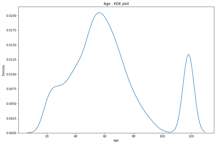
If we set these ages to NaN, we see that they correspond to users for whom the gender and income is also missing. There’s about 2000 of these people for whom we have basically no user data. We’ll just drop them from the DataFrame.
| Column | Count |
|---|---|
| Gender | 2175 |
| Age | 2175 |
| Became Member On | 0 |
| Income | 2175 |
| Account Age | 0 |
Data Exploration
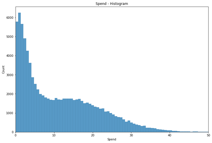
If we do a bar plot of a user’s spend in the training period we see that the modal spend is only a few dollars - likely the cost of a single coffee. It is not uncommon however for users to spend in the 10-20 dollar range, and higher spend become increasingly uncommon.
A plot of income versus spend reveals some clear clustering.
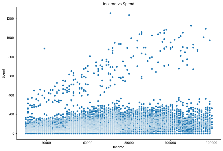
There’s a very noticeable group of people with very high spend, especially compared to income. Although we are unlikely to be able to use raw spend and transaction data to predict offer uptake (since this data is partially a function of offers completed), these kinds of groupings might be useful both for the model itself as well as development of heuristics.
If someone where to go to Starbucks every day and pay the mean transaction spend each day they would pay about $400. Most of the people in the high spend cluster spent more than this. We’ll call this group Big Spenders.
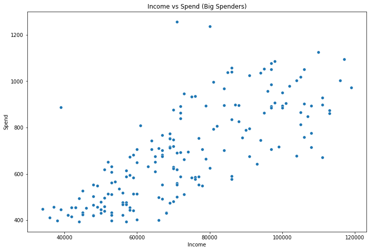
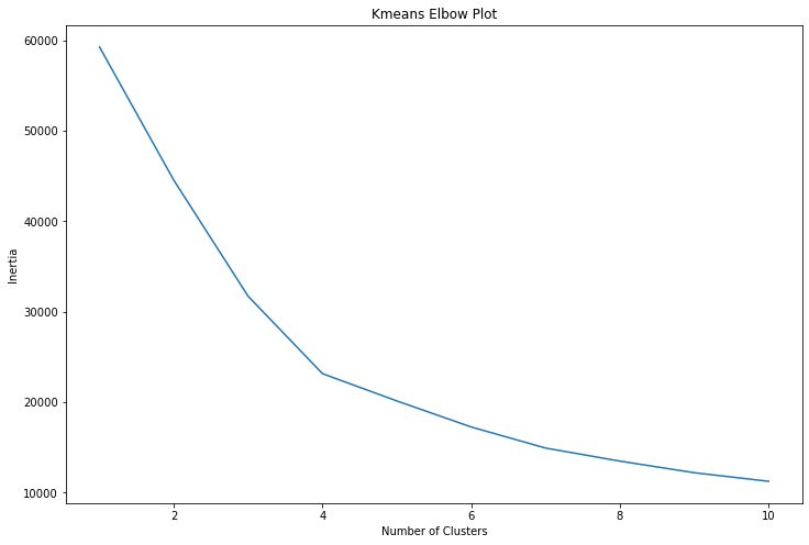
To identify this group more methodically we can use K-means clustering. The data points we use for the clustering are
- Income
- Mean Spend
- Number of Transactions
- Spend/Income
We see from an elbow plot that the optimum number of clusters is four.
Once we do the clustering we see that cluster 3 corresponds to the expected Big Spender cluster.
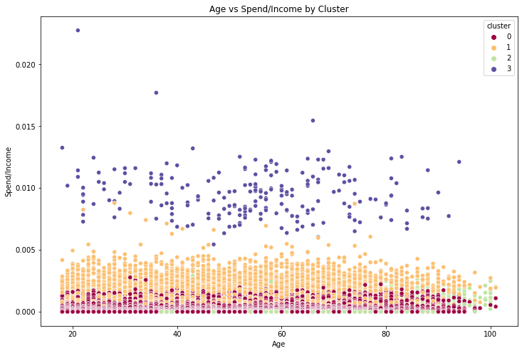
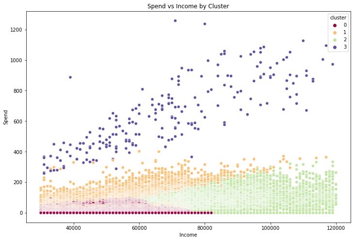
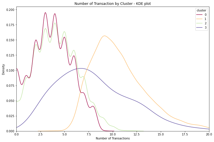
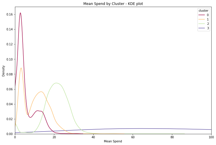
These clusters all have quite different spending patterns, exactly as we wanted. The big_spender cluster in particular is very different, having totally different mean spend distribution and a distinct number of transaction distribution as well.
Offer Completion
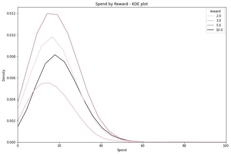
We can see that the impact of rewards are not uniform in how they affect spend. Users claiming a reward tend to spend significantly more than those who are not completing an offer - for which the average spend is about 10 dollars and the modal spend about 2 dollars 50.
| Reward | Mean Spend |
|---|---|
| 0 | 10.6 |
| 2 | 20.0 |
| 3 | 17.5 |
| 5 | 21.2 |
| 10 | 23.2 |
We can also ask what proportion of offers are completed.
| Name | Viewed | Completed |
|---|---|---|
| bogo,10,10,5 | 0.956432 | 0.478789 |
| bogo,10,10,7 | 0.884469 | 0.511061 |
| bogo,5,5,5 | 0.953036 | 0.600229 |
| bogo,5,5,7 | 0.519257 | 0.570684 |
| discount,2,10,10 | 0.967377 | 0.694608 |
| discount,2,10,7 | 0.521993 | 0.529399 |
| discount,3,7,7 | 0.957282 | 0.684844 |
| discount,5,20,10 | 0.332224 | 0.425150 |
| informational,0,0,3 | 0.814573 | 0.112565 |
| informational,0,0,4 | 0.477578 | 0.129372 |
| All | 0.736746 | 0.472950 |
We can also think of this in terms of total rewards earned versus rewards offered. In both cases we see that about 50% of offers are completed/rewards are earned.
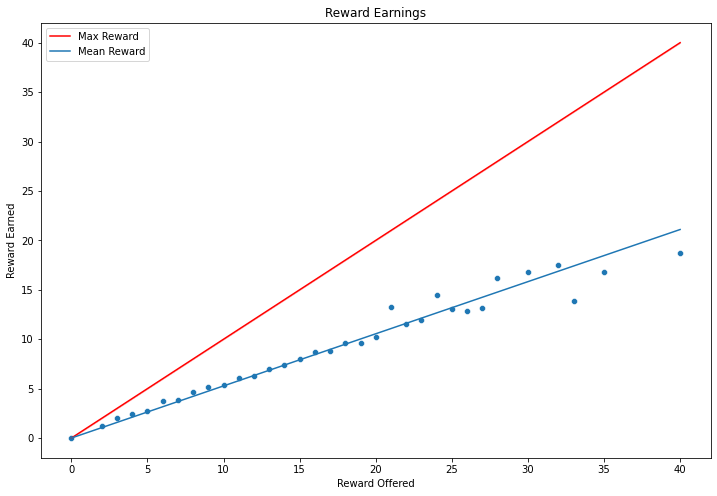
The poor fit towards the end is likely due, at least in part, to fewer people being offered such large max rewards.
P_testing Offer Effectiveness
We can also ask whether these offers have a meaningful or (statistically) significant impact on user spending. To this end employ a t-test between offer recipients during the offer period and those who have received no offer in this same period. The table of results is as follows. The p_x columns contain $-log(p)$ where $p$ is the p_value output of the t-test. A score above 3 can be considered significant.
| p_age | p_income | p_total-cost | total-cost | p_total | offered_total | null_total | p_mean | offered_mean | null_mean | p_count | offered_count | null_count | |
|---|---|---|---|---|---|---|---|---|---|---|---|---|---|
| discount,2,10,10 | 0.373081 | 0.513743 | 251.415865 | 30.652512 | 283.408413 | 46.875874 | 14.223363 | 36.634555 | 13.352046 | 8.858298 | inf | 3.280471 | 1.043826 |
| discount,3,7,7 | 0.472075 | 0.418224 | 187.476382 | 18.569828 | 249.576284 | 33.467657 | 11.897829 | 32.359681 | 11.840403 | 8.185221 | inf | 2.492615 | 0.867023 |
| bogo,5,5,5 | 0.627717 | 0.307679 | 92.664772 | 12.317879 | 177.398431 | 26.940110 | 9.622231 | 52.153454 | 11.919873 | 6.976287 | inf | 1.866667 | 0.705882 |
| discount,2,10,7 | 0.888283 | 0.627830 | 80.655369 | 12.179083 | 107.848849 | 26.076912 | 11.897829 | 21.634059 | 11.161493 | 8.185221 | 377.954748 | 1.737208 | 0.867023 |
| discount,5,20,10 | 0.367586 | 0.735100 | 53.657970 | 11.965843 | 104.198406 | 31.189206 | 14.223363 | 19.425179 | 12.090161 | 8.858298 | 332.601467 | 1.965403 | 1.043826 |
| bogo,10,10,7 | 0.949229 | 0.115336 | 48.955730 | 9.915389 | 184.972483 | 31.813218 | 11.897829 | 29.090939 | 11.862773 | 8.185221 | inf | 2.413184 | 0.867023 |
| bogo,5,5,7 | 0.725452 | 0.584020 | 40.097766 | 7.913657 | 101.293686 | 24.811486 | 11.897829 | 14.263930 | 10.484330 | 8.185221 | 372.677502 | 1.742637 | 0.867023 |
| informational,0,0,3 | 0.952612 | 0.920038 | 108.007086 | 6.960021 | 108.007086 | 13.918947 | 6.958925 | 49.624650 | 8.354929 | 5.289228 | 420.722524 | 1.116625 | 0.522302 |
| bogo,10,10,5 | 0.178025 | 0.665663 | 34.850332 | 6.925740 | 189.016236 | 26.547971 | 9.622231 | 59.501045 | 11.383595 | 6.976287 | inf | 1.933272 | 0.705882 |
| informational,0,0,4 | 0.489737 | 0.747444 | 59.748068 | 5.720949 | 59.748068 | 13.865758 | 8.144809 | 25.925570 | 8.166071 | 6.139471 | 220.613258 | 1.012556 | 0.597345 |
The key figures here are that age and income seem similarly distributed across null and test groups; and that the $p_{total-cost}$ value is always large. This means that we can reject the hypothesis that the total spend of people to whom the offer was made was lower than the total spend of those who it wasn’t plus the monetary value of the offer itself. That is the impact of the offer was both significant and meaningful. Although these tests were aggregated into one number for each offer, the information used was only from the periods in which the offer was active.
Noticeably there was an increase in both mean spend and number of transactions among offered groups.
| Offer | Increase in Spend/ Duration | Reward | Difficulty | Duration | Offer_type | Mobile | Social | Web | |
|---|---|---|---|---|---|---|---|---|---|
| discount,2,10,10 | 3.065251 | 2 | 10 | 10 | discount | 1.0 | 1.0 | 1.0 | 1.0 |
| discount,3,7,7 | 2.652833 | 3 | 7 | 7 | discount | 1.0 | 1.0 | 1.0 | 1.0 |
| bogo,5,5,5 | 2.463576 | 5 | 5 | 5 | bogo | 1.0 | 1.0 | 1.0 | 1.0 |
| informational,0,0,3 | 2.320007 | 0 | 0 | 3 | informational | 1.0 | 1.0 | 1.0 | 0.0 |
| discount,2,10,7 | 1.739869 | 2 | 10 | 7 | discount | 1.0 | 1.0 | 0.0 | 1.0 |
| informational,0,0,4 | 1.430237 | 0 | 0 | 4 | informational | 1.0 | 1.0 | 0.0 | 1.0 |
| bogo,10,10,7 | 1.416484 | 10 | 10 | 7 | bogo | 1.0 | 1.0 | 1.0 | 0.0 |
| bogo,10,10,5 | 1.385148 | 10 | 10 | 5 | bogo | 1.0 | 1.0 | 1.0 | 1.0 |
| discount,5,20,10 | 1.196584 | 5 | 20 | 10 | discount | 1.0 | 0.0 | 0.0 | 1.0 |
| bogo,5,5,7 | 1.130522 | 5 | 5 | 7 | bogo | 1.0 | 1.0 | 0.0 | 1.0 |
While all the measures are deemed effective by our p_tests, there does seem to be differences in performance. Roughly speaking it looks like the 2,10,10 discount performs best, but comparing the offers like this is on shaky statistical footing. There may be other factors impacting performance, e.g. people might be more likely to buy coffee on a Monday, so offers which include a (or multiple) Mondays might get a boost.
Offer Classification
Random Forest Model - Offer by offer prediction
We will use a random forest classifier to predict whether a user will view or complete a given offer. Initially a model is fitted for each offer individually so only information about the user is relevant.
The data points used for the predictions are:
- Age (Int)
- Income (Int)
- Account age (Int)
- Big Spender Cluster (Bool)
- Cluster 2 (Bool)
- Male (Bool)
- Female (Bool)
- Mean Spend (Float)
The Cluster 0 and Cluster 1 data points are not used because they don’t improve the predictive power of the model.
In addition to the base classifier SMOTE is used to resample the data due to the imbalanced nature of the data set. Further the parameters are tuned with a grid search carried out independently for each offer. The parameter grid is generated by
param_grid={
    'criterion':['gini', 'entropy'],
    'min_samples_split':np.logspace(-5,-1,5),
    'min_samples_leaf':np.logspace(-6,-2,5),
}
Other than these parameters the default sklearn options were used. This was largely due to computational limits. With a different model for each offer running extensive grid searches is very time consuming, especially on basic hardware.
The problem is a mulit-output classification one and therefore we can choose to run the grid search for a single multioutput classifier, or the search can be run on each output separately. The second option was chosen as it improved performance and with only two outputs it isn’t too difficult to do so. The grids evaluated parameters by their f1-score across three cross validations.
The best parameters are then used to refit a model on the entire test set.
We collect the results for each offer below.
| Type | Offer | Metric | Not Viewed | Viewed | Not Completed | Completed |
|---|---|---|---|---|---|---|
| bogo | bogo,10,10,5 | f1-score | 0.470588 | 0.976853 | 0.799180 | 0.843949 |
| precision | 0.758621 | 0.960902 | 0.899654 | 0.776557 | ||
| recall | 0.341085 | 0.993343 | 0.718894 | 0.924150 | ||
| support | 129.000000 | 2103.000000 | 1085.000000 | 1147.000000 | ||
| bogo,10,10,7 | f1-score | 0.651357 | 0.957582 | 0.793616 | 0.855714 | |
| precision | 0.829787 | 0.933168 | 0.850236 | 0.817647 | ||
| recall | 0.536082 | 0.983307 | 0.744066 | 0.897498 | ||
| support | 291.000000 | 1917.000000 | 969.000000 | 1239.000000 | ||
| bogo,5,5,5 | f1-score | 0.375000 | 0.978962 | 0.661710 | 0.805556 | |
| precision | 0.642857 | 0.965422 | 0.651220 | 0.813084 | ||
| recall | 0.264706 | 0.992888 | 0.672544 | 0.798165 | ||
| support | 102.000000 | 2109.000000 | 794.000000 | 1417.000000 | ||
| bogo,5,5,7 | f1-score | 0.675980 | 0.690486 | 0.683483 | 0.816823 | |
| precision | 0.674460 | 0.691976 | 0.655530 | 0.837491 | ||
| recall | 0.677507 | 0.689003 | 0.713927 | 0.797151 | ||
| support | 1107.000000 | 1164.000000 | 797.000000 | 1474.000000 | ||
| discount | discount,2,10,10 | f1-score | 0.503704 | 0.984566 | 0.704268 | 0.877370 |
| precision | 0.809524 | 0.973133 | 0.689552 | 0.885204 | ||
| recall | 0.365591 | 0.996270 | 0.719626 | 0.869674 | ||
| support | 93.000000 | 2145.000000 | 642.000000 | 1596.000000 | ||
| discount,2,10,7 | f1-score | 0.691812 | 0.691812 | 0.683951 | 0.812317 | |
| precision | 0.685506 | 0.698236 | 0.708440 | 0.795977 | ||
| recall | 0.698236 | 0.685506 | 0.661098 | 0.829341 | ||
| support | 1077.000000 | 1097.000000 | 838.000000 | 1336.000000 | ||
| discount,3,7,7 | f1-score | 0.488550 | 0.984693 | 0.597179 | 0.840965 | |
| precision | 0.761905 | 0.974231 | 0.532123 | 0.883615 | ||
| recall | 0.359551 | 0.995381 | 0.680357 | 0.802243 | ||
| support | 89.000000 | 2165.000000 | 560.000000 | 1694.000000 | ||
| discount,5,20,10 | f1-score | 0.882175 | 0.758763 | 0.733211 | 0.743363 | |
| precision | 0.885445 | 0.753070 | 0.850587 | 0.656250 | ||
| recall | 0.878930 | 0.764543 | 0.644301 | 0.857143 | ||
| support | 1495.000000 | 722.000000 | 1237.000000 | 980.000000 | ||
| informational | informational,0,0,3 | f1-score | 0.693997 | 0.944073 | 0.933436 | 0.510397 |
| precision | 0.858696 | 0.912099 | 0.887152 | 0.828221 | ||
| recall | 0.582310 | 0.978369 | 0.984816 | 0.368852 | ||
| support | 407.000000 | 1803.000000 | 1844.000000 | 366.000000 | ||
| informational,0,0,4 | f1-score | 0.709934 | 0.691404 | 0.943843 | 0.472813 | |
| precision | 0.715939 | 0.685289 | 0.900962 | 0.854701 | ||
| recall | 0.704028 | 0.697630 | 0.991010 | 0.326797 | ||
| support | 1142.000000 | 1055.000000 | 1891.000000 | 306.000000 |
Recall on classes with low support is predictably poor despite the resampling. This is a limitation of the data, there’s only so much we can do to improve the performance here. That being said, we can also try building a model to classify on multiple offers at once. In particular we can start to use information about the offer such as whether it was sent by email. We can do this either for all offers at once or by offer type.
Random Forest Model - Alternative prediction methods
Once again a grid search was run on each output before a model was refit on the entire training set. This time the parameter grid was slightly expanded since there are fewer models to build.
param_grid={
    'criterion':['gini', 'entropy'],
    'min_samples_split':np.logspace(-5,-1,5),
    'min_samples_leaf':np.logspace(-6,-2,5),
}
Because the Completed class is less unbalanced for some of these aggregated sets, so SMOTE sampling was less clearly needed. The performance differences were very small however, and it was much easier to pick a single option. With a bit of work this could have been included as parameter in the grid search however, which would have been a good option to eke out a bit of extra performance if one of these methods were to be chosen.
To compare these models we consider their combined performance by offer type as well as their overall performance. A breakdown by offer is also possible but it is difficult to read such a large table and meaningfully interpret the results.
| Type | Metric | Method | Not Viewed | Viewed | Not Completed | Completed |
|---|---|---|---|---|---|---|
| bogo | f1-score | All at once | 0.521869 | 0.915683 | 0.730182 | 0.830887 |
| Offer by offer | 0.645097 | 0.927438 | 0.738933 | 0.829567 | ||
| Type by type | 0.567692 | 0.879088 | 0.731456 | 0.792449 | ||
| precision | All at once | 0.667304 | 0.881793 | 0.777090 | 0.800597 | |
| Offer by offer | 0.697857 | 0.913321 | 0.765207 | 0.811379 | ||
| Type by type | 0.487450 | 0.921516 | 0.688195 | 0.832916 | ||
| recall | All at once | 0.428484 | 0.952283 | 0.688615 | 0.863559 | |
| Offer by offer | 0.599754 | 0.941999 | 0.714403 | 0.848588 | ||
| Type by type | 0.679558 | 0.840395 | 0.780521 | 0.755732 | ||
| support | NaN | 1629.000000 | 7293.000000 | 3645.000000 | 5277.000000 | |
| discount | f1-score | All at once | 0.728989 | 0.881592 | 0.664318 | 0.818087 |
| Offer by offer | 0.786861 | 0.906455 | 0.687559 | 0.824842 | ||
| Type by type | 0.721246 | 0.856631 | 0.681159 | 0.804071 | ||
| precision | All at once | 0.743580 | 0.874098 | 0.699023 | 0.796653 | |
| Offer by offer | 0.800000 | 0.899968 | 0.706602 | 0.812565 | ||
| Type by type | 0.663415 | 0.896841 | 0.660832 | 0.819563 | ||
| recall | All at once | 0.714960 | 0.889215 | 0.632896 | 0.840706 | |
| Offer by offer | 0.774147 | 0.913036 | 0.669515 | 0.837496 | ||
| Type by type | 0.790123 | 0.819873 | 0.702777 | 0.789154 | ||
| support | NaN | 2754.000000 | 6129.000000 | 3277.000000 | 5606.000000 | |
| informational | f1-score | All at once | 0.606533 | 0.826797 | 0.917465 | 0.000000 |
| Offer by offer | 0.706242 | 0.852370 | 0.938692 | 0.493697 | ||
| Type by type | 0.612913 | 0.775327 | 0.901182 | 0.086047 | ||
| precision | All at once | 0.713537 | 0.775598 | 0.847515 | 0.000000 | |
| Offer by offer | 0.744103 | 0.831117 | 0.894112 | 0.839286 | ||
| Type by type | 0.587678 | 0.795145 | 0.849490 | 0.196809 | ||
| recall | All at once | 0.527437 | 0.885234 | 1.000000 | 0.000000 | |
| Offer by offer | 0.672046 | 0.874738 | 0.987952 | 0.349702 | ||
| Type by type | 0.640413 | 0.756473 | 0.959572 | 0.055060 | ||
| support | NaN | 1549.000000 | 2858.000000 | 3735.000000 | 672.000000 |
| Metric | Method | Not Viewed | Viewed | Not Completed | Completed |
|---|---|---|---|---|---|
| f1-score | All at once | 0.646922 | 0.886994 | 0.782560 | 0.800414 |
| Offer by offer | 0.728326 | 0.906261 | 0.797295 | 0.813419 | |
| Type by type | 0.649153 | 0.852142 | 0.776350 | 0.770578 | |
| precision | All at once | 0.719983 | 0.859092 | 0.784515 | 0.798587 |
| Offer by offer | 0.759517 | 0.893599 | 0.798119 | 0.812646 | |
| Type by type | 0.590551 | 0.889334 | 0.737625 | 0.814440 | |
| recall | All at once | 0.587323 | 0.916769 | 0.780614 | 0.802250 |
| Offer by offer | 0.699595 | 0.919287 | 0.796472 | 0.814193 | |
| Type by type | 0.720668 | 0.817936 | 0.819368 | 0.731199 | |
| support | NaN | 5932.000000 | 16280.000000 | 10657.000000 | 11555.000000 |
The Offer by Offer method is the clear winner here. It is the best in almost every case and never the worst. All at once often offers similar performance but performs really poorly in some areas, in particular predicting completion of informational offers and recall of Not Viewed is very poor. Type by Type does occasionally do better than Offer by Offer but is also often much worse, overall it the poorer choice.
That being said they offer a degree of flexibility that the offer by offer does not, there is no scope to estimate performance on untested offer combinations using this method. A Random Forest model may not be the best choice for this kind of prediction, however.
Alternative Model Testing
Just as a sanity check, we can see how other types of model perform to confirm the choice of a random forest was sensible. For speed and ease of comparison we use the models to predict against all the offers at once. We also don’t use a grid search and add a standard scaler to the Pipeline. The models tested are as follows. Only a quick reference was sought, so all models were run with their default setups. As usual this was also done to keep computational time down.
| Models | Initial |
|---|---|
| Logistic Regression | LR |
| Decision Tree Classifier | DTC |
| Linear Discriminant Analysis | LDA |
| Random Forest Classifier | RFC |
| K-Neighbours Classifier | KNC |
| Gaussian Naive Bayes | GNB |
| SGDClassifier | SGDC |
| Metric | Model | Not Viewed | Viewed | Not Completed | Completed |
|---|---|---|---|---|---|
| f1-score | RFC | 0.642572 | 0.878630 | 0.763706 | 0.771635 |
| KNC | 0.619437 | 0.872887 | 0.766370 | 0.773149 | |
| LR | 0.615140 | 0.868381 | 0.767676 | 0.770751 | |
| SGDC | 0.583110 | 0.853203 | 0.766043 | 0.760177 | |
| LDA | 0.638180 | 0.850885 | 0.740597 | 0.752376 | |
| DTC | 0.585024 | 0.844201 | 0.720325 | 0.708758 | |
| GNB | 0.591651 | 0.841299 | 0.710868 | 0.747883 | |
| precision | LDA | 0.588227 | 0.881745 | 0.727783 | 0.765238 |
| RFC | 0.678927 | 0.862939 | 0.745974 | 0.789779 | |
| GNB | 0.565759 | 0.856534 | 0.732862 | 0.728811 | |
| LR | 0.646131 | 0.854366 | 0.742439 | 0.797501 | |
| KNC | 0.663649 | 0.853886 | 0.746883 | 0.793245 | |
| DTC | 0.572651 | 0.851105 | 0.679883 | 0.755560 | |
| SGDC | 0.598368 | 0.845611 | 0.728064 | 0.803121 | |
| recall | RFC | 0.609912 | 0.894902 | 0.782303 | 0.754305 |
| KNC | 0.580748 | 0.892752 | 0.786901 | 0.754046 | |
| LR | 0.586986 | 0.882862 | 0.794689 | 0.745738 | |
| SGDC | 0.568611 | 0.860934 | 0.808201 | 0.721592 | |
| DTC | 0.597943 | 0.837408 | 0.765882 | 0.667417 | |
| GNB | 0.620027 | 0.826597 | 0.690157 | 0.767979 | |
| LDA | 0.697404 | 0.822113 | 0.753871 | 0.739939 |
As we can see a Random Forest Classifier is the best performing but both the K-Neighbours Classifier and Linear Regression Classifier offer similar performance, especially the former. Linear Regression in particular might be used to build a model which is more suited to predicting the performance of offers which have not been tested here.
Offer Decision Making
There are many ways we could make the decision on what offers to suggest. We could for example send any offer we think will be accepted. Here we will use a rough estimate of the gain from sending an offer, calculated as
Ideally we would replace $P(\text{not viewed})$ with $P(\text{not viewed} \mid \text{completed})$ but since estimation of whether an offer would be viewed was already fairly poor, I worried such an estimate would be very inaccurate.
Similarly reward is used as an estimate of the cost of providing the offer but it is not a perfect representative. It likely over-estimates the gain of discounts verses buy one get one free offers as the marginal cost of providing a second coffee is likely much lower than menu price.
We use this to pick the top three offers, with no more than two of each type, for each user.
The first few entries of the resulting DataFrame look like this.
| Person | 1st | 2nd | 3rd |
|---|---|---|---|
| ae6f43089b674728a50b8727252d3305 | discount,2,10,10 | bogo,10,10,5 | bogo,10,10,7 |
| ad1f0a409ae642bc9a43f31f56c130fc | discount,2,10,10 | discount,5,20,10 | bogo,10,10,5 |
| dce784e26f294101999d000fad9089bb | discount,2,10,10 | bogo,10,10,5 | discount,3,7,7 |
| 4d0ebb94a5a94fe6afd9350c7b1477e4 | discount,2,10,10 | discount,5,20,10 | bogo,10,10,5 |
| 7d7f271652d244f78b97c73cd734c553 | discount,5,20,10 | discount,2,10,10 | bogo,10,10,7 |
The discount,2,10,10 offer appears a lot in these rows. In fact we can count the number of times each offer is recommend and see this pattern holds in the rest of the DataFrame.
| Offer | Count |
|---|---|
| Bogo,10,10,7 | 6367 |
| Bogo,10,10,5 | 7518 |
| Bogo,5,5,7 | 0 |
| Bogo,5,5,5 | 1608 |
| Discount,5,20,10 | 8221 |
| Discount, 2,10,10 | 14607 |
| Discount,2,10,7 | 499 |
| Discount,3,7,7 | 5655 |
| Informational,0,0,4 | 0 |
| Informational,0,0,3 | 0 |
Conclusion
By far and away the most suggested offer is the 2,10,10 discount. This is also the best performing offer according to the tentative analysis in the p-testing section which is reassuring. The decision making algorithm is a little crude. It could be improved with access to more data, like the cost of providing offer rewards. Given a larger data set we might also be able to make estimates of the conditional probabilities needed to give a more accurate estimate of offer gain.
Ultimately it isn’t really possible to give a good measure of how effective this strategy is. This would require real world testing. An experiment could be run where different groups are given offers according to different strategies e.g. the method above, random allocation, everyone gets the same, etc. Performance could then be compared across groups and the best strategy could be found.
As well as running a one off experiment this could be done as a continuous process. Since the rewards app collects all the relevant data models could be constantly updated and different A/B tests run each month with tweaked offer strategies in order to keep improving the performance.
We can of course evaluate the model performance according the the f1-score we highlighted as a metric at the beginning. It’s difficult to say whether a model is good or bad in a vacuum, based only on its scores, but the overall performance was respectable. The the grid search implementation, the SMOTE sampling and the decision to build a separate model for each offer all improved the scores from the base Random Forest Implementation. In particular this increased the Not Viewed f1-score (which was the worst) from about 0.64 to 0.73. This was driven by better scores in both recall and precision.
There were also noticeable, if less dramatic, improvements in the other f1-scores.
It is also clear both from the poor performance of the model itself and the predictions made that informational offers have not been handled well. They are very different in nature to the other offers and there is room for more exploration of when and how to use these kinds of offers.
As mentioned at the beginning, what is really missing here is a good estimate of the impact on a user’s spend of receiving an offer. It is clear from the p-testing section that there is a benefit to sending out an offer beyond just that realised by an additional purchase to redeem the offer. For example the 2,10,10 discount led to an increase in mean number of transactions from 1 to 3, and the total spend rose by over $30 as a result.
There is also scope for development of additional heuristics. Partly these depend on company goals. For example we might want to avoid sending offers to big spenders on the basis we think they are unlikely to be swayed by them. Conversely we might want to send offers to regular users, even if they would make the purchases anyways, in order to increase brand loyalty and retain their custom.
Some key areas for future work are as follows:
- Better identify underlying relationships in the data
- Who are social media offers most effective on?
- Do any users react negatively to receiving offers?
- Investigate the use of ensemble models to improve performance
- Train alternative models like Linear Regression and K-means and combine the output
- Train models in different ways like Type by Type or All at Once and combine